Python for NLP: Creating Multi-Data-Type Classification Models with Keras

This is the 18th article in my series of articles on Python for NLP. In my previous article, I explained how to create a deep learning-based movie sentiment analysis model using Python's Keras library. In that article, we saw how we can perform sentiment analysis of user reviews regarding different movies on IMDB. We used the text of the review to predict the sentiment.

However, in text classification tasks, we can also make use of the non-textual information to classify the text. For instance, gender may have an impact on the sentiment of the review. Furthermore, nationalities may affect the public opinion about a particular movie. Therefore, this associated info, also known as metadata can also be used to improve accuracy of the statistical model.

In this article, we will build upon the concepts that we studied in the last two articles and will see how to create a text classification system that classifies user reviews regarding different business, into one of the three predefined categories i.e. "good", "bad", and "average". However, in addition to the text of the review, we will use the associated metadata of the review to perform classification. Since we have two different types of inputs i.e. textual input and numerical input, we need to create a multiple inputs model. We will be using Keras Functional API since it supports multiple inputs and multiple output models.

After reading this article, you will be able to create a deep learning model in Keras that is capable of accepting multiple inputs, concatenating the two outputs and then performing classification or regression using the aggregated input.

• The Dataset
• Creating a Model with Text Inputs Only
• Creating a Model with Meta Information Only
• Creating a Model with Multiple Inputs
• Final Thoughts and Improvements

Before we dive into the details of creating such a model, let's first briefly review the dataset that we are going to use.

The Dataset

The dataset for this article can be downloaded from this Kaggle link. The dataset contains multiple files, but we are only interested in the yelp_review.csv file. The file contains more than 5.2 million reviews about different businesses, including restaurants, bars, dentists, doctors, beauty salons, etc. For our purposes we will only be using the first 50,000 records to train our model. Download the dataset to your local machine.

Let's first import all the libraries that we will be using in this article before importing the dataset.

from numpy import array
from keras.preprocessing.text import one_hot
from keras.preprocessing.sequence import pad_sequences
from keras.models import Sequential
from keras.layers.core import Activation, Dropout, Dense
from keras.layers import Flatten, LSTM
from keras.layers import GlobalMaxPooling1D
from keras.models import Model
from keras.layers.embeddings import Embedding
from sklearn.model_selection import train_test_split
from keras.preprocessing.text import Tokenizer
from keras.layers import Input
from keras.layers.merge import Concatenate

import pandas as pd
import numpy as np
import re

As a first step, we need to load the dataset. The following script does that:

yelp_reviews = pd.read_csv("/content/drive/My Drive/yelp_review_short.csv")

The dataset contains a column Stars that contains ratings for different businesses. The "Stars" column can have values between 1 and 5. We will simplify our problem by converting the numerical values for the reviews into categorical ones. We will add a new column reviews_score to our dataset. If the user review has a value of 1 in the Stars column, the reviews_score column will have a string value bad. If the rating is 2 or 3 in the Stars column, the reviews_score column will contain a value average. Finally a review rating of 4 or 5 will have a corresponding value of good in the reviews_score column.

The following script performs this preprocessing:

bins = [0,1,3,5]
review_names = ['bad', 'average', 'good']
yelp_reviews['reviews_score'] = pd.cut(yelp_reviews['stars'], bins, labels=review_names)

Next, we will remove all the NULL values from our dataframe and will print the shape and the header of the dataset.

yelp_reviews.isnull().values.any()

print(yelp_reviews.shape)

yelp_reviews.head()

In the output you will see (50000,10), which means that our dataset contains 50,000 records with 10 columns. The header of the yelp_reviews dataframe looks like this:

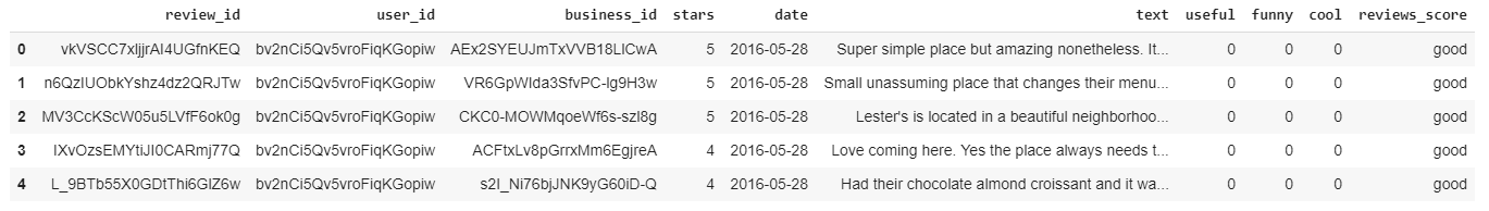
You can see the 10 columns that our dataframe contains, including the newly added reviews_score column. The text column contains the text of the review while the useful column contains numerical value that represents the count of the people who found the review useful. Similarly, the funny and cool columns contain the counts of people who found reviews funny or cool, respectively.

Let's randomly choose a review. If you look at the 4th review (review with index 3), it has 4 stars and hence it is marked as good. Let's view the complete text of this review:

print(yelp_reviews["text"][3])

The output looks like this:

Love coming here. Yes the place always needs the floor swept but when you give out  peanuts in the shell how won't it always be a bit dirty.

The food speaks for itself, so good. Burgers are made to order and the meat is put on the grill when you order your sandwich. Getting the small burger just means 1 patty, the regular is a 2 patty burger which is twice the deliciousness.

Getting the Cajun fries adds a bit of spice to them and whatever size you order they always throw more fries (a lot more fries) into the bag.

You can clearly see that this is a positive review.

Let's now plot the number of good, average, and bad reviews.

import seaborn as sns

sns.countplot(x='reviews_score', data=yelp_reviews)

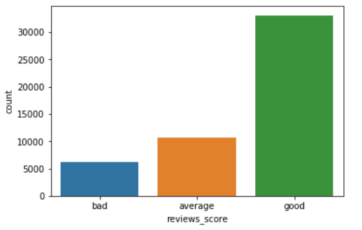
It is evident from the above plot that the majority of the reviews are good, followed by the average reviews. The number of negative reviews is very small.

We have preprocessed our data and now we will create three models in this article. The first model will only use text inputs for predicting whether a review is good, average, or bad. In the second model, we will not use text. We will only use the meta information such as useful, funny, and cool to predict the sentiment of the review. Finally, we will create a model that accepts multiple inputs i.e. text and meta information for text classification.

Creating a Model with Text Inputs Only

The first step is to define a function that cleans the textual data.

def preprocess_text(sen):

    # Remove punctuations and numbers
    sentence = re.sub('[^a-zA-Z]', ' ', sen)

    # Single character removal
    sentence = re.sub(r"\s+[a-zA-Z]\s+", ' ', sentence)

    # Removing multiple spaces
    sentence = re.sub(r'\s+', ' ', sentence)

    return sentence

Since we are only using text in this model, we will filter all the text reviews and store them in the list. The text reviews will be cleaned using the preprocess_text function, which removes punctuations and numbers from the text.

X = []
sentences = list(yelp_reviews["text"])
for sen in sentences:
    X.append(preprocess_text(sen))

y = yelp_reviews['reviews_score']

Our X variable here contains the text reviews while the y variable contains the corresponding reviews_score values. The reviews_score column has data in the text format. We need to convert the text to a one-hot encoded vector. We can use the to_categorical method from the keras.utils module. However, first we have to convert the text into integer labels using the LabelEncoder function from the sklearn.preprocessing module.

from sklearn import preprocessing

# label_encoder object knows how to understand word labels.
label_encoder = preprocessing.LabelEncoder()

# Encode labels in column 'species'.
y = label_encoder.fit_transform(y)

Let's now divide our data into testing and training sets:

X_train, X_test, y_train, y_test = train_test_split(X, y, test_size=0.20, random_state=42)

Now we can convert both the training and test labels into one-hot encoded vectors:

from keras.utils import to_categorical
y_train = to_categorical(y_train)
y_test = to_categorical(y_test)

I explained in my article on word embeddings that textual data has to be converted into some sort of numeric form before it can be used by statistical algorithms like machine and deep learning models. One way to convert text to numbers is via word embeddings. If you are unaware of how to implement word embeddings via Keras, I highly recommend that you read this article before moving on to the next sections of the code.

The first step in word embeddings is to convert the words into their corresponding numeric indexes. To do so, we can use the Tokenizer class from the Keras.preprocessing.text module.

tokenizer = Tokenizer(num_words=5000)
tokenizer.fit_on_texts(X_train)

X_train = tokenizer.texts_to_sequences(X_train)
X_test = tokenizer.texts_to_sequences(X_test)

Sentences can have different lengths, and therefore the sequences returned by the Tokenizer class also consist of variable lengths. We specify that the maximum length of the sequence will be 200 (although you can try any number). For the sentences having length less than 200, the remaining indexes will be padded with zeros. For the sentences having length greater than 200, the remaining indexes will be truncated.

Look at the following script:

vocab_size = len(tokenizer.word_index) + 1

maxlen = 200

X_train = pad_sequences(X_train, padding='post', maxlen=maxlen)
X_test = pad_sequences(X_test, padding='post', maxlen=maxlen)

Next, we need to load the built-in GloVe word embeddings.

from numpy import array
from numpy import asarray
from numpy import zeros

embeddings_dictionary = dict()

for line in glove_file:
    records = line.split()
    word = records[0]
    vector_dimensions = asarray(records[1:], dtype='float32')
    embeddings_dictionary [word] = vector_dimensions

glove_file.close()

Finally, we will create an embedding matrix where rows will be equal to the number of words in the vocabulary (plus 1). The number of columns will be 100 since each word in the GloVe word embeddings that we loaded is represented as a 100 dimensional vector.

embedding_matrix = zeros((vocab_size, 100))
for word, index in tokenizer.word_index.items():
    embedding_vector = embeddings_dictionary.get(word)
    if embedding_vector is not None:
        embedding_matrix[index] = embedding_vector

Once the word embedding step is completed, we are ready to create our model. We will be using Keras' functional API to create our model. Though single input models like the one we are creating now can be developed using sequential API as well, but as in the next section we are going to develop a multiple input model that can only be developed using Keras functional API, we will stick to functional API in this section too.

We will create a very simple model with one input layer (embedding layer), one LSTM layer with 128 neurons and one dense layer that will act as the output layer as well. Since we have 3 possible outputs, the number of neurons will be 3 and the activation function will be softmax. We will use the categorical_crossentropy as our loss function and adam as the optimization function.

deep_inputs = Input(shape=(maxlen,))
embedding_layer = Embedding(vocab_size, 100, weights=[embedding_matrix], trainable=False)(deep_inputs)
LSTM_Layer_1 = LSTM(128)(embedding_layer)
dense_layer_1 = Dense(3, activation='softmax')(LSTM_Layer_1)
model = Model(inputs=deep_inputs, outputs=dense_layer_1)

model.compile(loss='categorical_crossentropy', optimizer='adam', metrics=['acc'])

Let's print the summary of our model:

print(model.summary())

_________________________________________________________________
Layer (type)                 Output Shape              Param #
=================================================================
input_1 (InputLayer)         (None, 200)               0
_________________________________________________________________
embedding_1 (Embedding)      (None, 200, 100)          5572900
_________________________________________________________________
lstm_1 (LSTM)                (None, 128)               117248
_________________________________________________________________
dense_1 (Dense)              (None, 3)                 387
=================================================================
Total params: 5,690,535
Trainable params: 117,635
Non-trainable params: 5,572,900

Finally, lets print the block diagram of our neural network:

from keras.utils import plot_model
plot_model(model, to_file='model_plot1.png', show_shapes=True, show_layer_names=True)

The file model_plot1.png will be created in your local file path. If you open the image, it will look like this:

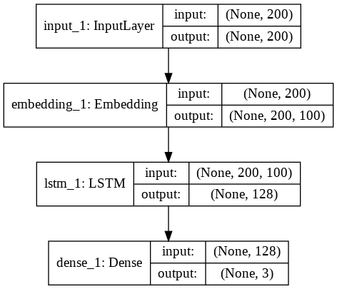
You can see that the model has 1 input layer, 1 embedding layer, 1 LSTM, and one dense layer which serves as the output layer as well.

Let's now train our model:

history = model.fit(X_train, y_train, batch_size=128, epochs=10, verbose=1, validation_split=0.2)

The model will be trained on 80% of the train data and will be validated on 20% of the train data. The results for the 10 epochs is as follows:

Train on 32000 samples, validate on 8000 samples
Epoch 1/10
32000/32000 [==============================] - 81s 3ms/step - loss: 0.8640 - acc: 0.6623 - val_loss: 0.8356 - val_acc: 0.6730
Epoch 2/10
32000/32000 [==============================] - 80s 3ms/step - loss: 0.8508 - acc: 0.6618 - val_loss: 0.8399 - val_acc: 0.6690
Epoch 3/10
32000/32000 [==============================] - 84s 3ms/step - loss: 0.8461 - acc: 0.6647 - val_loss: 0.8374 - val_acc: 0.6726
Epoch 4/10
32000/32000 [==============================] - 82s 3ms/step - loss: 0.8288 - acc: 0.6709 - val_loss: 0.7392 - val_acc: 0.6861
Epoch 5/10
32000/32000 [==============================] - 82s 3ms/step - loss: 0.7444 - acc: 0.6804 - val_loss: 0.6371 - val_acc: 0.7311
Epoch 6/10
32000/32000 [==============================] - 83s 3ms/step - loss: 0.5969 - acc: 0.7484 - val_loss: 0.5602 - val_acc: 0.7682
Epoch 7/10
32000/32000 [==============================] - 82s 3ms/step - loss: 0.5484 - acc: 0.7623 - val_loss: 0.5244 - val_acc: 0.7814
Epoch 8/10
32000/32000 [==============================] - 86s 3ms/step - loss: 0.5052 - acc: 0.7866 - val_loss: 0.4971 - val_acc: 0.7950
Epoch 9/10
32000/32000 [==============================] - 84s 3ms/step - loss: 0.4753 - acc: 0.8032 - val_loss: 0.4839 - val_acc: 0.7965
Epoch 10/10
32000/32000 [==============================] - 82s 3ms/step - loss: 0.4539 - acc: 0.8110 - val_loss: 0.4622 - val_acc: 0.8046

You can see that the final training accuracy of the model is 81.10% while validation accuracy is 80.46. The difference is very small and therefore we assume that our model is not overfitting on the training data.

Let's now evaluate the performance of our model on test set:

score = model.evaluate(X_test, y_test, verbose=1)

print("Test Score:", score[0])
print("Test Accuracy:", score[1])

The output looks like this:

10000/10000 [==============================] - 37s 4ms/step
Test Score: 0.4592904740810394
Test Accuracy: 0.8101

Finally, let's plot the values for loss and accuracy for both training and testing sets:

import matplotlib.pyplot as plt

plt.plot(history.history['acc'])
plt.plot(history.history['val_acc'])

plt.title('model accuracy')
plt.ylabel('accuracy')
plt.xlabel('epoch')
plt.legend(['train','test'], loc='upper left')
plt.show()

plt.plot(history.history['loss'])
plt.plot(history.history['val_loss'])

plt.title('model loss')
plt.ylabel('loss')
plt.xlabel('epoch')
plt.legend(['train','test'], loc='upper left')
plt.show()

You should see the following two plots:

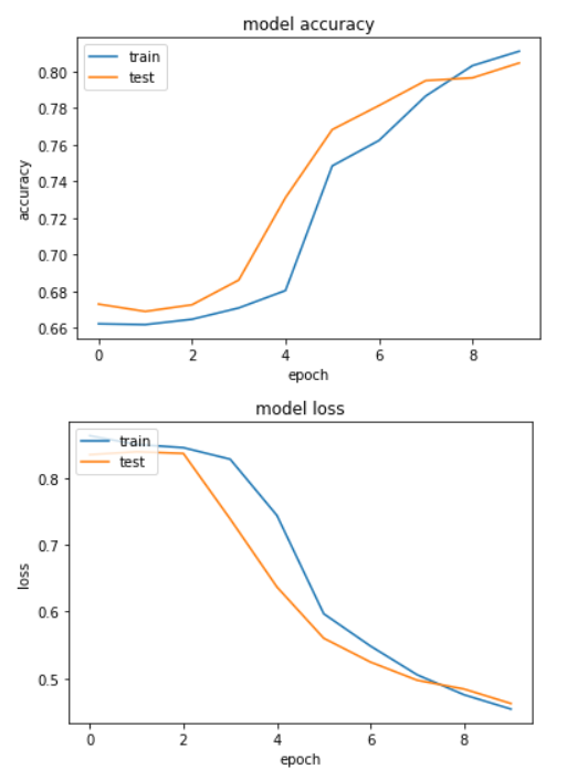
You can see the lines for both training and testing accuracies and losses are pretty close to each other which means that the model is not overfitting.

Creating a Model with Meta Information Only

In this section, we will create a classification model that uses information from the useful, funny, and cool columns of the yelp reviews. Since the data for these columns is well structured and doesn't contain any sequential or spatial pattern, we can use simple densely connected neural networks to make predictions.

Let's plot the average counts for useful, funny, and cool reviews against the review score.

import seaborn as sns
sns.barplot(x='reviews_score', y='useful', data=yelp_reviews)

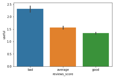
From the output, you can see that the average count for reviews marked as useful is the highest for the bad reviews, followed by the average reviews and the good reviews.

Let's now plot the average count for funny reviews:

sns.barplot(x='reviews_score', y='funny', data=yelp_reviews)

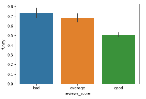
The output shows that again, the average count for reviews marked as funny is highest for the bad reviews.

Finally, let's plot the average value for the cool column against the reviews_score column. We expect that the average count for the cool column will be the highest for good reviews since people often mark positive or good reviews as cool:

sns.barplot(x='reviews_score', y='cool', data=yelp_reviews)

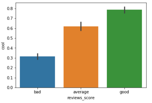
As expected, the average cool count for the good reviews is the highest. From this information, we can safely assume that the count values for useful, funny, and cool columns have some correlation with the reviews_score columns. Therefore, we will try to use the data from these three columns to train our algorithm that predicts the value for the reviews_score column.

Let's filter these three columns from our dataset:

yelp_reviews_meta = yelp_reviews[['useful', 'funny', 'cool']]

X = yelp_reviews_meta.values

y = yelp_reviews['reviews_score']

Next, we will convert our labels into one-hot encoded values and then split our data into train and test sets:

from sklearn import preprocessing

# label_encoder object knows how to understand word labels.
label_encoder = preprocessing.LabelEncoder()

# Encode labels in column 'species'.
y = label_encoder.fit_transform(y)

X_train, X_test, y_train, y_test = train_test_split(X, y, test_size=0.20, random_state=42)

from keras.utils import to_categorical
y_train = to_categorical(y_train)
y_test = to_categorical(y_test)

The next step is to create our model. Our model will consist of four layers (you can try any number): the input layer, two dense hidden layers with 10 neurons and ReLU activation functions, and finally an output dense layer with 3 neurons and softmax activation function. The loss function and optimizer will be categorical_crossentropy and adam, respectively.

The following script defines the model:

input2 = Input(shape=(3,))
dense_layer_1 = Dense(10, activation='relu')(input2)
dense_layer_2 = Dense(10, activation='relu')(dense_layer_1)
output = Dense(3, activation='softmax')(dense_layer_2)

model = Model(inputs=input2, outputs=output)
model.compile(loss='categorical_crossentropy', optimizer='adam', metrics=['acc'])

Let's print the summary of the model:

print(model.summary())

_________________________________________________________________
Layer (type)                 Output Shape              Param #
=================================================================
input_1 (InputLayer)         (None, 3)                 0
_________________________________________________________________
dense_1 (Dense)              (None, 10)                40
_________________________________________________________________
dense_2 (Dense)              (None, 10)                110
_________________________________________________________________
dense_3 (Dense)              (None, 3)                 33
=================================================================
Total params: 183
Trainable params: 183
Non-trainable params: 0

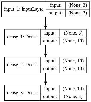
Finally, the block diagram for the model can be created via the following script:

from keras.utils import plot_model
plot_model(model, to_file='model_plot2.png', show_shapes=True, show_layer_names=True)

Now, if you open the model_plot2.png file from your local file path, it looks like this:

Let's now train the model and print the accuracy and loss values for each epoch:

history = model.fit(X_train, y_train, batch_size=16, epochs=10, verbose=1, validation_split=0.2)

Train on 32000 samples, validate on 8000 samples
Epoch 1/10
32000/32000 [==============================] - 8s 260us/step - loss: 0.8429 - acc: 0.6649 - val_loss: 0.8166 - val_acc: 0.6734
Epoch 2/10
32000/32000 [==============================] - 7s 214us/step - loss: 0.8203 - acc: 0.6685 - val_loss: 0.8156 - val_acc: 0.6737
Epoch 3/10
32000/32000 [==============================] - 7s 217us/step - loss: 0.8187 - acc: 0.6685 - val_loss: 0.8150 - val_acc: 0.6736
Epoch 4/10
32000/32000 [==============================] - 7s 220us/step - loss: 0.8183 - acc: 0.6695 - val_loss: 0.8160 - val_acc: 0.6740
Epoch 5/10
32000/32000 [==============================] - 7s 227us/step - loss: 0.8177 - acc: 0.6686 - val_loss: 0.8149 - val_acc: 0.6751
Epoch 6/10
32000/32000 [==============================] - 7s 219us/step - loss: 0.8175 - acc: 0.6686 - val_loss: 0.8157 - val_acc: 0.6744
Epoch 7/10
32000/32000 [==============================] - 7s 216us/step - loss: 0.8172 - acc: 0.6696 - val_loss: 0.8145 - val_acc: 0.6733
Epoch 8/10
32000/32000 [==============================] - 7s 214us/step - loss: 0.8175 - acc: 0.6689 - val_loss: 0.8139 - val_acc: 0.6734
Epoch 9/10
32000/32000 [==============================] - 7s 215us/step - loss: 0.8169 - acc: 0.6691 - val_loss: 0.8160 - val_acc: 0.6744
Epoch 10/10
32000/32000 [==============================] - 7s 216us/step - loss: 0.8167 - acc: 0.6694 - val_loss: 0.8138 - val_acc: 0.6736

From the output, you can see that our model doesn't converge and accuracy values remain between 66 and 67 across all the epochs.

Let's see how the model performs on test set:

score = model.evaluate(X_test, y_test, verbose=1)

print("Test Score:", score[0])
print("Test Accuracy:", score[1])

10000/10000 [==============================] - 0s 34us/step
Test Score: 0.8206425309181213
Test Accuracy: 0.6669

We can print the loss and accuracy values for training and test sets via the following script:

import matplotlib.pyplot as plt

plt.plot(history.history['acc'])
plt.plot(history.history['val_acc'])

plt.title('model accuracy')
plt.ylabel('accuracy')
plt.xlabel('epoch')
plt.legend(['train','test'], loc='upper left')
plt.show()

plt.plot(history.history['loss'])
plt.plot(history.history['val_loss'])

plt.title('model loss')
plt.ylabel('loss')
plt.xlabel('epoch')
plt.legend(['train','test'], loc='upper left')
plt.show()

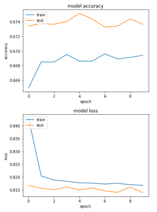
From the output, you can see that accuracy values are relatively lower. Hence, we can say that our model is under-fitting. The accuracy can be increased by increasing the number of dense layers or by increasing the number of epochs, however I will leave that to you.

Let's move on to the final and most important section of this article where we will use multiple inputs of different types to train our model.

Creating a Model with Multiple Inputs

In the previous sections, we saw how to train deep learning models using either textual data or meta information. What if we want to combine textual information with meta information and use that as input to our model? We can do so using the Keras functional API. In this section we will create two sub-models.

The first submodel will accept textual input in the form of text reviews. This submodel will consist of an input shape layer, an embedding layer, and an LSTM layer of 128 neurons. The second submodel will accept input in the form of meta information from the useful, funny, and cool columns. The second submodel also consists of three layers. An input layer and two dense layers.

The output from the LSTM layer of the first submodel and the output from the second dense layer of the second submodel will be concatenated together and will be used as concatenated input to another dense layer with 10 neurons. Finally, the output dense layer will have three neurons corresponding to each review type.

Let's see how we can create such a concatenated model.

First we have to create two different types of inputs. To do so, we will divide our data into a feature set and label set, as shown below:

X = yelp_reviews.drop('reviews_score', axis=1)

y = yelp_reviews['reviews_score']

The X variable contains the feature set, whereas the y variable contains the label set. We need to convert our labels into one-hot encoded vectors. We can do so using the label encoder and the to_categorical function of the keras.utils module. We will also divide our data into training and feature sets.

from sklearn import preprocessing

# label_encoder object knows how to understand word labels.
label_encoder = preprocessing.LabelEncoder()

# Encode labels in column 'species'.
y = label_encoder.fit_transform(y)

X_train, X_test, y_train, y_test = train_test_split(X, y, test_size=0.20, random_state=42)

from keras.utils import to_categorical
y_train = to_categorical(y_train)
y_test = to_categorical(y_test)

Now our label set is in the required form. Since there will be only one output, therefore we don't need to process our label set. However, there will be multiple inputs to the model. Therefore, we need to preprocess our feature set.

Let's first create preproces_text function that will be used to preprocess our dataset:

def preprocess_text(sen):

    # Remove punctuations and numbers
    sentence = re.sub('[^a-zA-Z]', ' ', sen)

    # Single character removal
    sentence = re.sub(r"\s+[a-zA-Z]\s+", ' ', sentence)

    # Removing multiple spaces
    sentence = re.sub(r'\s+', ' ', sentence)

    return sentence

As a first step, we will create textual input for the training and test set. Look at the following script:

X1_train = []
sentences = list(X_train["text"])
for sen in sentences:
    X1_train.append(preprocess_text(sen))

Now X1_train contains the textual input for the training set. Similarly, the following script preprocess textual input data for test set:

X1_test = []
sentences = list(X_test["text"])
for sen in sentences:
    X1_test.append(preprocess_text(sen))

Now we need to convert textual input for the training and test sets into numeric form using word embeddings. The following script does that:

tokenizer = Tokenizer(num_words=5000)
tokenizer.fit_on_texts(X1_train)

X1_train = tokenizer.texts_to_sequences(X1_train)
X1_test = tokenizer.texts_to_sequences(X1_test)

vocab_size = len(tokenizer.word_index) + 1

maxlen = 200

X1_train = pad_sequences(X1_train, padding='post', maxlen=maxlen)
X1_test = pad_sequences(X1_test, padding='post', maxlen=maxlen)

We will again use GloVe word embeddings for creating word vectors:

from numpy import array
from numpy import asarray
from numpy import zeros

embeddings_dictionary = dict()

glove_file = open('/content/drive/My Drive/glove.6B.100d.txt', encoding="utf8")

for line in glove_file:
    records = line.split()
    word = records[0]
    vector_dimensions = asarray(records[1:], dtype='float32')
    embeddings_dictionary[word] = vector_dimensions

glove_file.close()

embedding_matrix = zeros((vocab_size, 100))
for word, index in tokenizer.word_index.items():
    embedding_vector = embeddings_dictionary.get(word)
    if embedding_vector is not None:
        embedding_matrix[index] = embedding_vector

We have preprocessed our textual input. The second input type is the meta information in the useful, funny, and cool columns. We will filter these columns from the feature set to create meta input for training the algorithms. Look at the following script:

X2_train = X_train[['useful', 'funny', 'cool']].values
X2_test = X_test[['useful', 'funny', 'cool']].values

Let's now create our two input layers. The first input layer will be used to input the textual input and the second input layer will be used to input meta information from the three columns.

input_1 = Input(shape=(maxlen,))

input_2 = Input(shape=(3,))

You can see that the first input layer input_1 is used for the textual input. The shape size has been set to the shape of the input sentence. For the second input layer, the shape corresponds to three columns.

Let's now create the first submodel that accepts data from first input layer:

embedding_layer = Embedding(vocab_size, 100, weights=[embedding_matrix], trainable=False)(input_1)
LSTM_Layer_1 = LSTM(128)(embedding_layer)

Similarly, the following script creates a second submodel that accepts input from the second input layer:

dense_layer_1 = Dense(10, activation='relu')(input_2)
dense_layer_2 = Dense(10, activation='relu')(dense_layer_1)

We now have two sub-models. What we want to do is concatenate the output from the first submodel with the output from the second submodel. The output from the first submodel is the output from the LSTM_Layer_1 and similarly, the output from the second submodel is the output from the dense_layer_2. We can use the Concatenate class from the keras.layers.merge module to concatenate two inputs.

The following script creates our final model:

concat_layer = Concatenate()([LSTM_Layer_1, dense_layer_2])
dense_layer_3 = Dense(10, activation='relu')(concat_layer)
output = Dense(3, activation='softmax')(dense_layer_3)
model = Model(inputs=[input_1, input_2], outputs=output)

You can see that now our model has a list of inputs with two items. The following script compiles the model and prints its summary:

model.compile(loss='categorical_crossentropy', optimizer='adam', metrics=['acc'])
print(model.summary())

The model summary is as follows:

Layer (type)                    Output Shape         Param #     Connected to
==================================================================================================
input_1 (InputLayer)            (None, 200)          0
__________________________________________________________________________________________________
input_2 (InputLayer)            (None, 3)            0
__________________________________________________________________________________________________
embedding_1 (Embedding)         (None, 200, 100)     5572900     input_1[0][0]
__________________________________________________________________________________________________
dense_1 (Dense)                 (None, 10)           40          input_2[0][0]
__________________________________________________________________________________________________
lstm_1 (LSTM)                   (None, 128)          117248      embedding_1[0][0]
__________________________________________________________________________________________________
dense_2 (Dense)                 (None, 10)           110         dense_1[0][0]
__________________________________________________________________________________________________
concatenate_1 (Concatenate)     (None, 138)          0           lstm_1[0][0]
                                                                 dense_2[0][0]
__________________________________________________________________________________________________
dense_3 (Dense)                 (None, 10)           1390        concatenate_1[0][0]
__________________________________________________________________________________________________
dense_4 (Dense)                 (None, 3)            33          dense_3[0][0]
==================================================================================================
Total params: 5,691,721
Trainable params: 118,821
Non-trainable params: 5,572,900

Finally, we can plot the complete network model using the following script:

from keras.utils import plot_model
plot_model(model, to_file='model_plot3.png', show_shapes=True, show_layer_names=True)

If you open the model_plot3.png file, you should see the following network diagram:

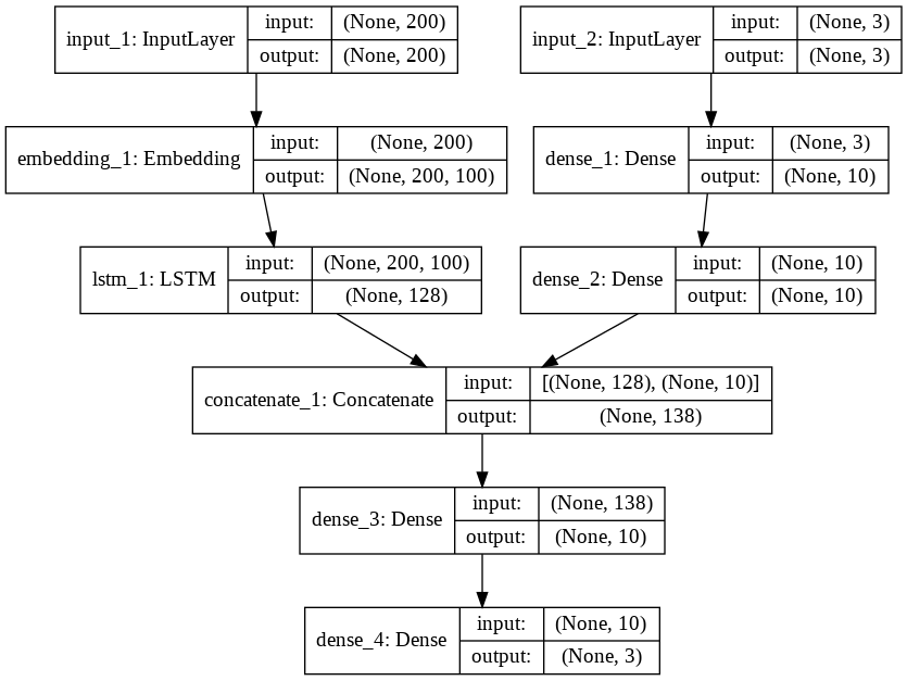
The above figure clearly explains how we have concatenated multiple inputs into one input to create our model.

Let's now train our model and see the results:

history = model.fit(x=[X1_train, X2_train], y=y_train, batch_size=128, epochs=10, verbose=1, validation_split=0.2)

Here is the result for the 10 epochs:

Train on 32000 samples, validate on 8000 samples
Epoch 1/10
32000/32000 [==============================] - 155s 5ms/step - loss: 0.9006 - acc: 0.6509 - val_loss: 0.8233 - val_acc: 0.6704
Epoch 2/10
32000/32000 [==============================] - 154s 5ms/step - loss: 0.8212 - acc: 0.6670 - val_loss: 0.8141 - val_acc: 0.6745
Epoch 3/10
32000/32000 [==============================] - 154s 5ms/step - loss: 0.8151 - acc: 0.6691 - val_loss: 0.8086 - val_acc: 0.6740
Epoch 4/10
32000/32000 [==============================] - 155s 5ms/step - loss: 0.8121 - acc: 0.6701 - val_loss: 0.8039 - val_acc: 0.6776
Epoch 5/10
32000/32000 [==============================] - 154s 5ms/step - loss: 0.8027 - acc: 0.6740 - val_loss: 0.7467 - val_acc: 0.6854
Epoch 6/10
32000/32000 [==============================] - 155s 5ms/step - loss: 0.6791 - acc: 0.7158 - val_loss: 0.5764 - val_acc: 0.7560
Epoch 7/10
32000/32000 [==============================] - 154s 5ms/step - loss: 0.5333 - acc: 0.7744 - val_loss: 0.5076 - val_acc: 0.7881
Epoch 8/10
32000/32000 [==============================] - 154s 5ms/step - loss: 0.4857 - acc: 0.7973 - val_loss: 0.4849 - val_acc: 0.7970
Epoch 9/10
32000/32000 [==============================] - 154s 5ms/step - loss: 0.4697 - acc: 0.8034 - val_loss: 0.4709 - val_acc: 0.8024
Epoch 10/10
32000/32000 [==============================] - 154s 5ms/step - loss: 0.4479 - acc: 0.8123 - val_loss: 0.4592 - val_acc: 0.8079

To evaluate our model, we will have to pass both the test inputs to the evaluate function as shown below:

score = model.evaluate(x=[X1_test, X2_test], y=y_test, verbose=1)

print("Test Score:", score[0])
print("Test Accuracy:", score[1])

Here are the result:

10000/10000 [==============================] - 18s 2ms/step
Test Score: 0.4576087875843048
Test Accuracy: 0.8053

Our test accuracy is 80.53%, which is slightly less than our first model that uses textual input only. This shows that meta information in yelp_reviews is not very useful for sentiment prediction.

Anyways, now you know how to create multiple input models for text classification in Keras!

Finally, let's now print the loss and accuracy for training and test sets:

import matplotlib.pyplot as plt

plt.plot(history.history['acc'])
plt.plot(history.history['val_acc'])

plt.title('model accuracy')
plt.ylabel('accuracy')
plt.xlabel('epoch')
plt.legend(['train','test'], loc='upper left')
plt.show()

plt.plot(history.history['loss'])
plt.plot(history.history['val_loss'])

plt.title('model loss')
plt.ylabel('loss')
plt.xlabel('epoch')
plt.legend(['train','test'], loc='upper left')
plt.show()

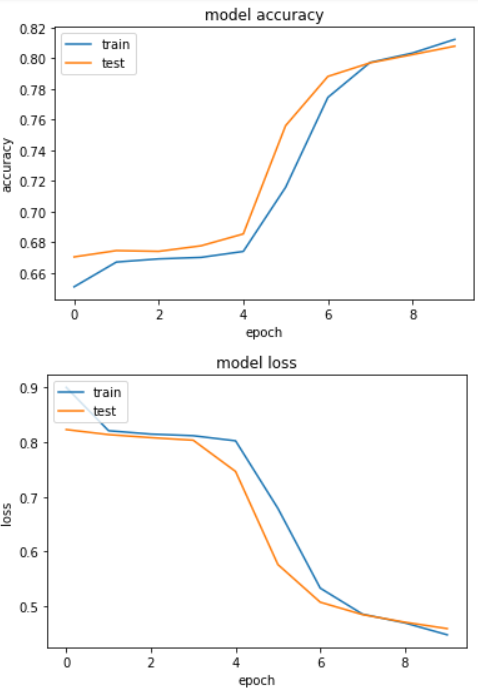
You can see that the differences for loss and accuracy values are minimal between the training and test sets, hence our model is not overfitting.

Final Thoughts and Improvements

In this article, we built a very simple neural network since the purpose of the article is to explain how to create a deep learning model that accepts multiple inputs of different types.

Following are some of the tips that you can follow to further improve the performance of the text classification model:

1. We only used 50,000, out of 5.2 million records in this article since we had hardware constraints. You can try training your model on a higher number of records and see if you can achieve better performance.
2. Try adding more LSTM and dense layers to the model. If the model overfits, try to add dropout.
3. Try to change the optimizer function and train the model with a higher number of epochs.

Please share your results along with the neural network configuration in the comments section. I would love to see how well you perform.